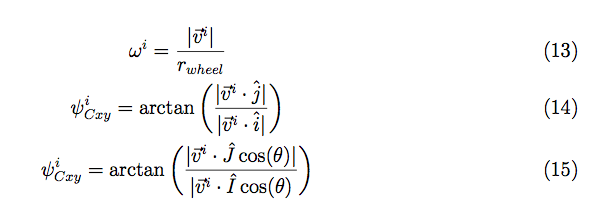
kinematics — Blog — David S Miller
Processing math: 100%
  • Portfolio
  • Aviation
  • Blog
  • About
Menu

David S Miller

  • Portfolio
  • Aviation
  • Blog
  • About
 +Y translation + CW rotation. Notice the skidding. If the X vel. were +, the motion would be correct. I hadn't fixed the wheel angles at this point though; those are still wrong.

+Y translation + CW rotation. Notice the skidding. If the X vel. were +, the motion would be correct. I hadn't fixed the wheel angles at this point though; those are still wrong.

 Pure translation in Q1. Notice the X velocity still seems to have the wrong sign.

Pure translation in Q1. Notice the X velocity still seems to have the wrong sign.

 I don't remember what this is. I don't think it worked...

I don't remember what this is. I don't think it worked...

 This looks correct, but it's not. If you try gradually reducing the rotation and keeping the translation the same, you'll notice something wrong. It's helpful to test limiting cases like this, by introducing things very slowly. 

This looks correct, but it's not. If you try gradually reducing the rotation and keeping the translation the same, you'll notice something wrong. It's helpful to test limiting cases like this, by introducing things very slowly. 

 I stopped doing the motion plots and just did a single snapshot with velocity vectors. You have to adjust the sign of the wheel velocity to get the vector pointing in the right direction.

I stopped doing the motion plots and just did a single snapshot with velocity vectors. You have to adjust the sign of the wheel velocity to get the vector pointing in the right direction.

 Here you can see all the wheels have the same velocity [vector] as each other, and as the body of the robot. Bingo.

Here you can see all the wheels have the same velocity [vector] as each other, and as the body of the robot. Bingo.

 Here's where I started trying to combine translation inputs and rotation inputs. Here the robot has a Y+ translation and a CCW rotation. The net result is a pure rotation about some point on the X axis.

Here's where I started trying to combine translation inputs and rotation inputs. Here the robot has a Y+ translation and a CCW rotation. The net result is a pure rotation about some point on the X axis.

 Now I'm combining X and Y translation with rotations. I repeated this for different quadrants (translation) and different rotation directions (CW,CCW). 

Now I'm combining X and Y translation with rotations. I repeated this for different quadrants (translation) and different rotation directions (CW,CCW). 

 You can see that the lower left wheel is on the largest radius of the orbit, and it has the highest speed. Good sign.

You can see that the lower left wheel is on the largest radius of the orbit, and it has the highest speed. Good sign.

 I went through each translational quadrant twice, one for each rotation direction (CW,CCW). 

I went through each translational quadrant twice, one for each rotation direction (CW,CCW). 

 One other verification I could do is making sure the normal lines from each wheel intersect at the same point. This is the orbital point I mentioned in the text below. 

One other verification I could do is making sure the normal lines from each wheel intersect at the same point. This is the orbital point I mentioned in the text below. 

success_5.png
success_4.png
success_3.png
success_2.png
 +Y translation + CW rotation. Notice the skidding. If the X vel. were +, the motion would be correct. I hadn't fixed the wheel angles at this point though; those are still wrong.  Pure translation in Q1. Notice the X velocity still seems to have the wrong sign.  I don't remember what this is. I don't think it worked...  This looks correct, but it's not. If you try gradually reducing the rotation and keeping the translation the same, you'll notice something wrong. It's helpful to test limiting cases like this, by introducing things very slowly.   I stopped doing the motion plots and just did a single snapshot with velocity vectors. You have to adjust the sign of the wheel velocity to get the vector pointing in the right direction.  Here you can see all the wheels have the same velocity [vector] as each other, and as the body of the robot. Bingo.  Here's where I started trying to combine translation inputs and rotation inputs. Here the robot has a Y+ translation and a CCW rotation. The net result is a pure rotation about some point on the X axis.  Now I'm combining X and Y translation with rotations. I repeated this for different quadrants (translation) and different rotation directions (CW,CCW).   You can see that the lower left wheel is on the largest radius of the orbit, and it has the highest speed. Good sign.  I went through each translational quadrant twice, one for each rotation direction (CW,CCW).   One other verification I could do is making sure the normal lines from each wheel intersect at the same point. This is the orbital point I mentioned in the text below.  success_5.pngsuccess_4.pngsuccess_3.pngsuccess_2.png

Kinematics of Wheeled Mobile Robots Pt. 3

April 14, 2016

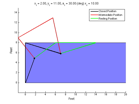
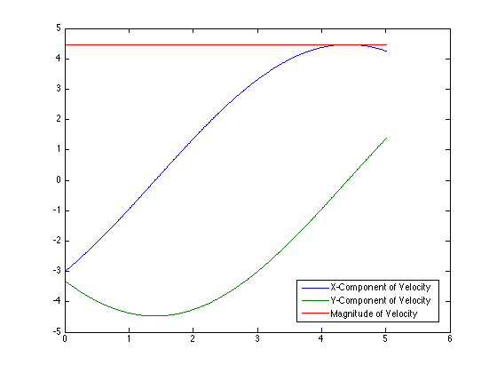
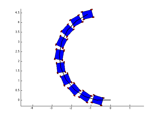
Our team finally got the robot moving and steering! Which means it's finally time for me to start the implementation process of the kinematic and control equations. To further verify and help prepare for the implementation, I made a little simulator in MATLAB to help visualize how the robot will move given certain (steady state) commands. Transient commands are a whole other issue, which I may discuss later. 

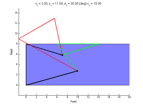
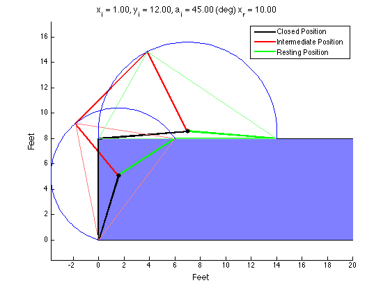
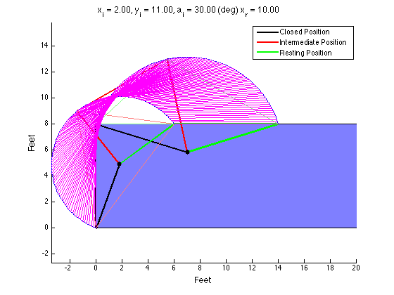
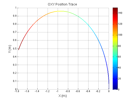
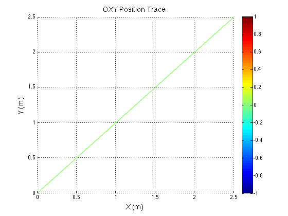
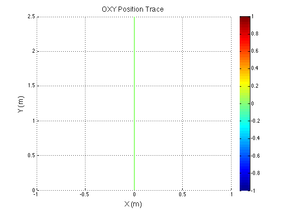
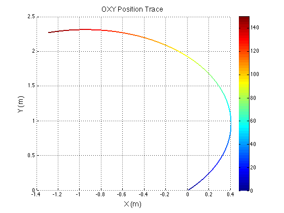
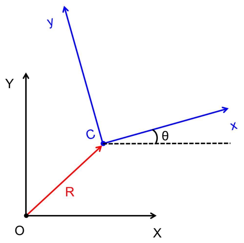
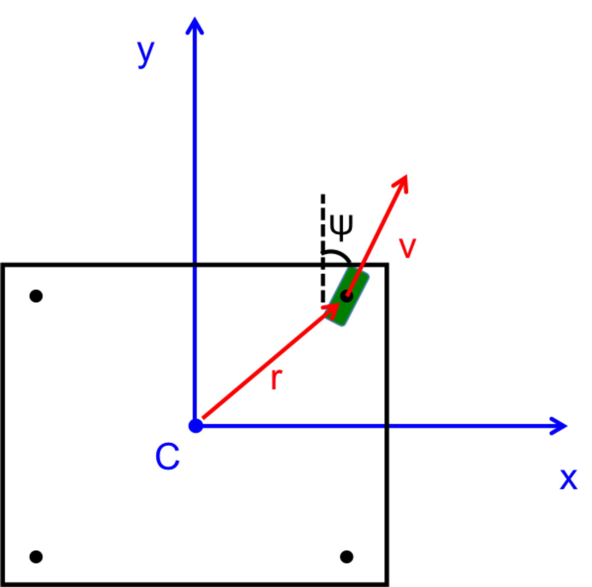
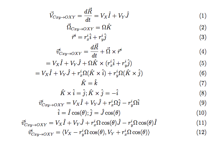
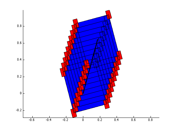
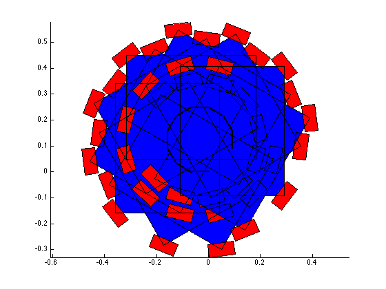
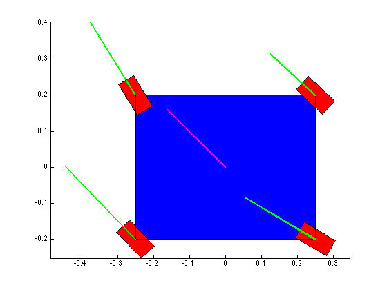
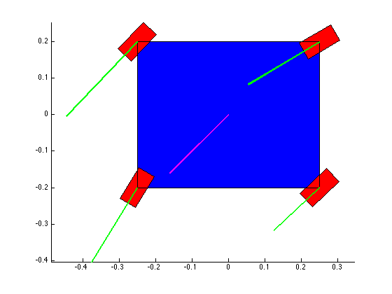
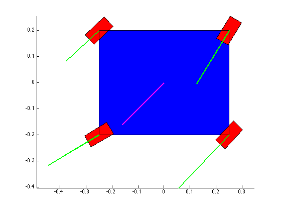
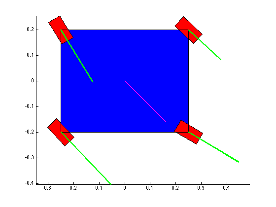
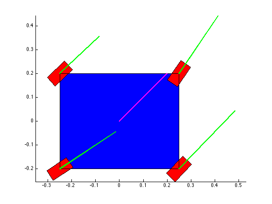
The structure of the top level code is simple. It defines the parameters of the robot and of the simulation, and calls the swerve_command function. This function performs the inverse kinematics and spits out the wheel angles and speeds, as well as the position (x, y, theta) information for that time step. Over several time steps, the robot will move. If steady state inputs are held, the wheel angles and speeds will remain constant, even if the robot itself is executing some curvilinear motion. The robot is plotted at each time step. To verify the wheel angles are correct, you need to visually confirm that the wheels are tangent to the path taken by the wheels in each snapshot. 

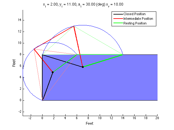
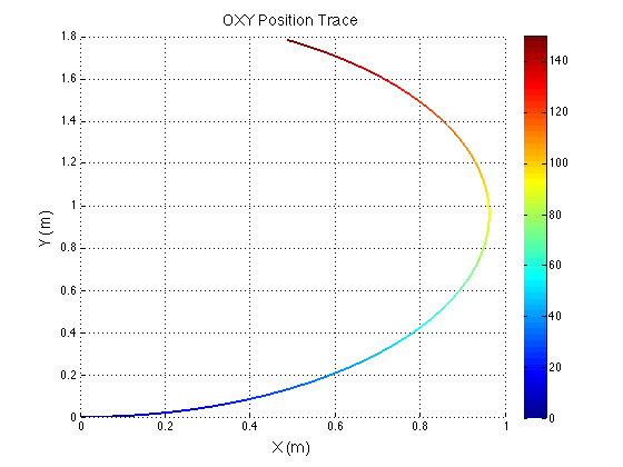
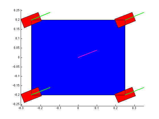
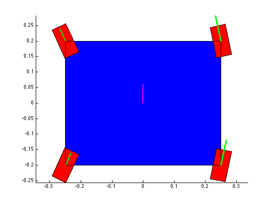
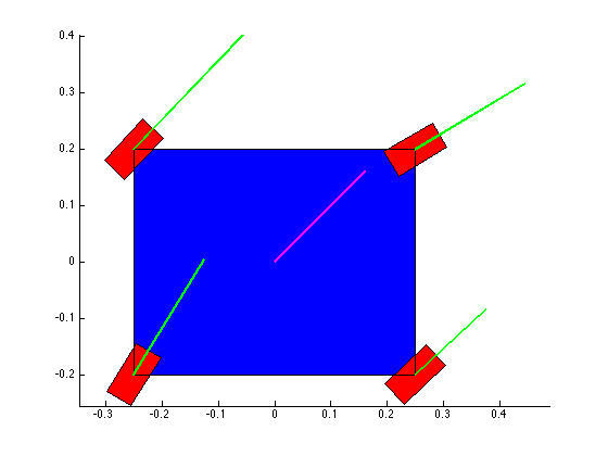
Confirming the wheel speeds is more difficult. For any type of pure translation all the wheel speeds just need to be the same. This has been confirmed. If there is any type of rotation involved, the wheels will orbiting some central point. If the location of the point is known, then the radius to each wheel can be found and using the omega = v/r equation you can confirm that all the angular speeds about that central point are equal. This is hard to do currently because we are normalizing all our speeds because they are simply throttling values which will be sent to the motors. We do not know exactly what speeds they will spin at. However, the ratios of the speeds are telling. What we know is that the wheels on the largest radius of the orbit must have the highest linear velocity, and the wheels on the smallest radius of the orbit must have the smallest linear velocity. This allows all the wheels to have the same angular velocity around that central point. As you can see from the photos, this phenomenon is evident by the colored velocity vectors. 

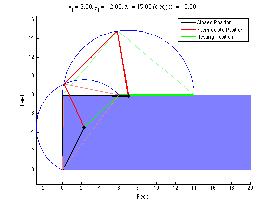
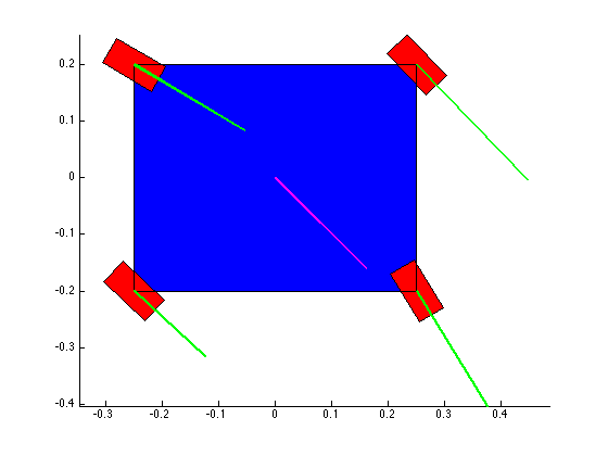
There is something funky going on with the way that the motion of the robot is plotted. The wheel angles and speeds look okay, but when I try to plot the motion some of the components of the motion (X and rotation) have the wrong sign and it looks like the robot is skidding across the floor. I haven't been able to figure out why that is yet. I have a feeling it's some kind of sign error but I haven't found it yet.


Open Issues:

  1. Figuring out how to update the wheel speeds and angles while moving (transient command inputs)

  2. Normalizing the wheel speed outputs to prevent speed commands to the motor from saturating

  3. Finding the little sign errors that are messing things up


Bonus:

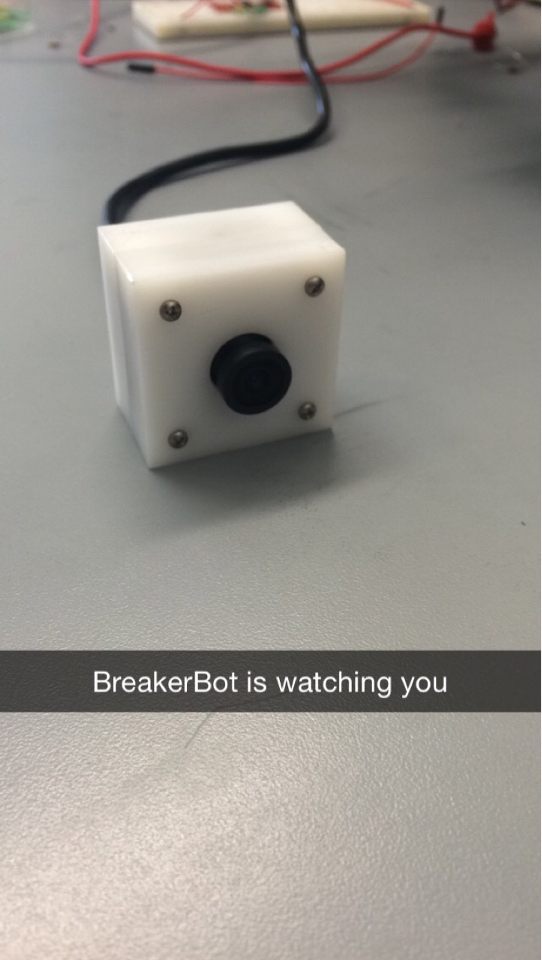
We also made a little case for the webcam BreakerBot will be using for the First Person View mode for remote operation. BreakerBot is watching you...

In Academic Projects, BreakerBot, MATLAB Projects Tags MATLAB, kinematics, Modeling
Comment
Share
 It appears that this mechanism is valid... But how can I be sure?

It appears that this mechanism is valid... But how can I be sure?

 By plotting arcs around the links I ensure they stay the same size throughout.

By plotting arcs around the links I ensure they stay the same size throughout.

 Here are some varying geometries that achieve the same goal.

Here are some varying geometries that achieve the same goal.

 This is when I was still debugging my code. You can clearly see each member changes length as it rotates, which cannot occur.

This is when I was still debugging my code. You can clearly see each member changes length as it rotates, which cannot occur.

 This geometry resulted in a bearing that was placed off the surface of the shipping container.

This geometry resulted in a bearing that was placed off the surface of the shipping container.

 One more geometry. The next question is, how can you optimize the linkage??

One more geometry. The next question is, how can you optimize the linkage??

 I tried plotting snapshots of the linkage but it didn't work so well. This is wrong because the magenta snapshots do not align with the red position.

I tried plotting snapshots of the linkage but it didn't work so well. This is wrong because the magenta snapshots do not align with the red position.

 It appears that this mechanism is valid... But how can I be sure?  By plotting arcs around the links I ensure they stay the same size throughout.  Here are some varying geometries that achieve the same goal.  This is when I was still debugging my code. You can clearly see each member changes length as it rotates, which cannot occur.  This geometry resulted in a bearing that was placed off the surface of the shipping container.  One more geometry. The next question is, how can you optimize the linkage??  I tried plotting snapshots of the linkage but it didn't work so well. This is wrong because the magenta snapshots do not align with the red position.

MATLAB Four-Bar Linkage Design

March 24, 2016

The Product Design class I am a TA for had an assignment to design a four-bar mechanism to move a lid on a shipping container up and over so that it rested on the top of the container during loading. There was extra credit awarded to those who could analytically arrive at a design using MATLAB (or some other language). I made my own solution for fun and to check student's solutions. I tried to get it to plot each snapshot (in magenta) but it was not correct and I didn't have time to figure it out. 

So, here's how to design a typical four-bar linkage:

  1. Define the desired locations of your coupler. You define two or three locations you want the coupler to travel through. My code only works with three locations.

  2. Find the locus of points that is equidistant from where the crank connects to the coupler in each position. If two coupler positions are defined, the locus will be an infinite line (think of the intersection of two circles; connecting the two points forms a line). If three coupler positions are defined, the locus collapses to a single point. This point also happens to be the circumcenter of the triangle formed by the three vertices the bearing must be equidistant from. The bearing must be placed on a point on the locus. If the locus is a single point, your job is done. If the locus is a line, you must select a point on that line to be your bearing location.

  3. Repeat step 2 for the points where the rocker connects to the coupler.

  4. Once you have the bearing locations for the crank and the rocker, you can easily calculate the lengths of each link.

In Academic Projects, Personal Projects, MATLAB Projects Tags MATLAB, kinematics, Mechanisms
Comment
Share
rstick_x-right_lstick_k-right_position-trace.png
lstick_y-up_lstick_k-right_position-trace.png
lstick_y-up_rstick_x-right_position-trace.png
lstick_y-up_position-trace.png
lstick_y-up_rstick_x-right_lstick_k-right_position-trace.png
pure_rotation.png
rstick_x-right_lstick_k-right_position-trace.pnglstick_y-up_lstick_k-right_position-trace.pnglstick_y-up_rstick_x-right_position-trace.pnglstick_y-up_position-trace.pnglstick_y-up_rstick_x-right_lstick_k-right_position-trace.pngpure_rotation.png

Kinematics of Wheeled Mobile Robots Pt. 2

February 29, 2016

I discovered a few minor issues with my previous derivation. I had not converted the unit vectors from one frame to the other correctly, and I left some of the expressions in the unit vectors of an inappropriate frame. MATLAB was used to verify the equations. Simple inputs were sent to the equations and various outputs were plotted for evaluation. The rainbow plots show the physical path of the robot in the XY plane. The color indicates the angle of rotation in degrees. The last graph shows my original eureka moment when I finally realized I fixed the problem. Previously, there was a cusp in the magnitude of velocity when it should have been constant. When I saw the constant red line, I knew I was on the right track. 

Because the control inputs are centered to the robot's frame, if you hold constant translational inputs with a rotation, the robot will end up taking a curved path. However if you hold constant translational inputs with no rotation, the robot will travel straight. This is shown by the graphs with no color change.

In BreakerBot, MATLAB Projects Tags robotics, kinematics, BreakerBot, MATLAB
Comment
Share
iso_perpective_render.JPG
iso_exp_perpective_render.JPG
 Opening

Opening

 Exposed Control Rods

Exposed Control Rods

iso_perpective_render.JPGiso_exp_perpective_render.JPG Opening  Exposed Control Rods

Isolating Pure Bending in Optical Fibers

February 20, 2016

One of the grad students from the nanophotonics lab I developed the microbend apparatus for contacted me regarding a question he had. He was trying to isolate bending and torsional loads in optical fibers to investigate their effects. Introducing pure bending in a fiber is difficult because the fibers have very little torsional stiffness. It's easy to eliminate bends to a twisted fiber by simply adding a bit of tension to the ends. But how do you eliminate twist? There is so little stiffness that you cannot rely on the restoring torque to eliminate small twists in the fiber. The current solution is to coil the fiber very loosely (coiling is just one very long continuous bend) whatever twist is inadvertently introduced by the act of coiling will distribute itself along the length of the entire fiber. In contrast, in fiber optic gyroscope winding, because the coils are so tight, the minor twists in the fiber get trapped between turns of the coil, leaving behind localized residual torsions in the fiber. 

The downside to a loose coil is that it is very hard to get each turn in the coil to the same diameter. A constant bending radius is required for accurate measurements. We decided to use an iris diaphragm mechanism to control the diameter of 6 pins, which the fiber will loosely be wrapped around as guides. This way, a very minimal amount of tension could be used to make sure the coils are all the same diameter, and the diameter can be adjusted using the iris mechanism. To go along with this, it would be helpful to have a limited slip fiber clamp and constant force spring loaded spool so the diameter could be adjusted either direction without having to manually pick up slack in the fiber or loosen the coils to reduce the tension. 

One other alternative to this 'loose coil' solution is to actively measure and correct the fiber twist. However, this method seems overly complex. It really depends on how much twist is tolerable. Once that is quantified, we will be able to determine what type of solution is required. I have a feeling the tolerance will not be so tight as to necessitate some type of active system. But I wonder if there is a better solution for an active system? Perhaps if instead of wrapping the fiber around pins, we could wrap it around an expanding cylinder controlled by the iris mechanism. But I have no idea how that could work. Time to start brainstorming...

In Personal Projects Tags Optics, Fiber, Mechanisms, kinematics, SolidWorks, Design
Comment
Share
 Reference frames.

Reference frames.

 Robot reference frame showing wheel locations and wheel angle.

Robot reference frame showing wheel locations and wheel angle.

 Coordinate frame transformation yields wheel velocities required to achieve specified motion.

Coordinate frame transformation yields wheel velocities required to achieve specified motion.

 Wheel rotational speeds and steering angles can be determined from the wheel velocity vectors.

Wheel rotational speeds and steering angles can be determined from the wheel velocity vectors.

 Position vectors from the center of the robot to each of the four wheels.

Position vectors from the center of the robot to each of the four wheels.

 Reference frames.  Robot reference frame showing wheel locations and wheel angle.  Coordinate frame transformation yields wheel velocities required to achieve specified motion.  Wheel rotational speeds and steering angles can be determined from the wheel velocity vectors.  Position vectors from the center of the robot to each of the four wheels.

Kinematics of Wheeled Mobile Robots

February 2, 2016

After many discussions, our group has decided that four-wheel drive simply does not permit adequate control of the robot for aligning with the circuit breaker cubicle. So we are reverting to our original drive train choice: swerve drive. Swerve drive is a holonomic locomotion system in which each wheel can pivot about its own vertical axis. Using a swerve drive, the robot will strafe sideways along the face of the circuit breaker cubicle, detecting the edges of the cubicle and using those edges to laterally align the robot. Then, the robot will perform an angular alignment to the face of the cubicle, and advance forward to extract the breaker. The angular alignment and subsequent forward motion would not have been possible with a four-wheel drive system; as the translation and rotation of the robot are coupled.

I derived the inverse kinematics of the robot for our computer engineers to use in their control algorithms. The derivation is quite simple mathematically, but it can easily get confusing to understand from a physical sense. I like to imagine what I would experience if I were sitting on the different points where the wheels are located on the robot. This helps me to see why certain terms are in the resulting equations and verify if the results make sense. 

PDF derivation of the kinematics.


In BreakerBot, MATLAB Projects Tags robotics, kinematics, BreakerBot
Comment
Share

Blogpost Search

Blogposts by Category

Select Category
  • Academic Projects
  • Aviation
  • BreakerBot
  • Engineering Education
  • Illusionist's Locket
  • MATLAB Projects
  • Machining Projects
  • Personal Projects

Archive

  • May 2024
  • December 2019
  • November 2019
  • September 2019
  • April 2017
  • January 2017
  • August 2016
  • May 2016
  • April 2016
  • March 2016
  • February 2016
  • January 2016
  • November 2015
  • October 2015
  • June 2015
  • April 2015
  • February 2015
  • January 2015

Copyright © David Miller 2019